First Power Analysis in R with MCPower

Every power analysis answers one of two questions:

1. Given a sample size, how much power do I have? — find_power
2. Given a power target, what sample size do I need? — find_sample_size

You only need to learn these two calls once. Every later rung changes the model and reuses them unchanged.

The model

We reuse the study from the landing page: does a treatment lift satisfaction, controlling for age?

• the formula satisfaction ~ treatment + age names the outcome and predictors;
• set_variable_type marks treatment as binary (a 0/1 group), leaving age continuous;
• set_effects sets the standardised effect we want to detect — see effect sizes for the 0.10 / 0.25 / 0.40 benchmarks.

target_test = "all" reports every predictor plus the overall F test; verbose = FALSE returns the result object instead of auto-printing, so we can call summary().

How much power at n = 120?

library(mcpower)

model <- MCPower$new("satisfaction ~ treatment + age")
model$set_variable_type("treatment=binary")
model$set_effects("treatment=0.5, age=0.3")

result <- model$find_power(sample_size = 120, target_test = "all", verbose = FALSE)
print(summary(result))

==================================================
  MCPower · Power Analysis
==================================================
formula: satisfaction ~ treatment + age
estimator: OLS  N=120  sims=1600  α=0.05  target=80%
effects: treatment=0.50, age=0.30

Per-test power
───────────────────────────────────
Test                 Power   Target
───────────────────────────────────
Overall F            97.0%      80%
treatment            77.4%      80%
age                  88.4%      80%
───────────────────────────────────

Power & 95% CI
───────────────────────────────────────────
Test                 Power           CI 95%
───────────────────────────────────────────
Overall F            97.0%   [96.0%, 97.7%]
treatment            77.4%   [75.3%, 79.4%]
age                  88.4%   [86.8%, 89.9%]
───────────────────────────────────────────
95% CIs are Monte-Carlo (Wilson), n_sims=1600.

Joint significance distribution
────────────────────────
k     Exactly   At least
────────────────────────
0        3.1%       100%
1       28.1%      96.9%
2       68.9%      68.9%
────────────────────────

Plots: plot(result) to view, plot(result, 'chart.png') to save.

treatment lands at 77.4% — below the 80% target — while age is comfortably powered at 88.4%. The joint significance distribution at the bottom gives the chance of detecting both effects in the same study (68.9%), which is necessarily lower than either alone.

What sample size reaches 80%?

find_sample_size simulates a grid of sample sizes (here 40 to 200 in steps of 20), fits a power curve through the results, and reports the n where that curve crosses the target:

library(mcpower)

model <- MCPower$new("satisfaction ~ treatment + age")
model$set_variable_type("treatment=binary")
model$set_effects("treatment=0.5, age=0.3")

result <- model$find_sample_size(target_test = "all", from_size = 40, to_size = 200, by = 20, verbose = FALSE)
print(summary(result))

==================================================
  MCPower · Power Analysis
==================================================
formula: satisfaction ~ treatment + age
estimator: OLS  N≥129  sims=1600  α=0.05  target=80%
effects: treatment=0.50, age=0.30

Required sample size per effect
───────────────────────────────
Test                 Required N
───────────────────────────────
Overall F                    70
treatment                   129
age                          96
───────────────────────────────

Required N & 95% CI
────────────────────────────────────────────
Test                 Required N       CI 95%
────────────────────────────────────────────
Overall F                    70     [66, 74]
treatment                   129   [122, 135]
age                          96    [91, 101]
────────────────────────────────────────────
Required N from the model-based crossing fit (isotonic); CI by Wilson band inversion, rounded outward.

Joint detection → required N (target 80%)
───────────────────────────────
Joint target         Required N
───────────────────────────────
≥ 2 of 2 tests              145
≥ 1 of 2 tests               65
───────────────────────────────

Plots: plot(result) to view, plot(result, 'chart.png') to save.

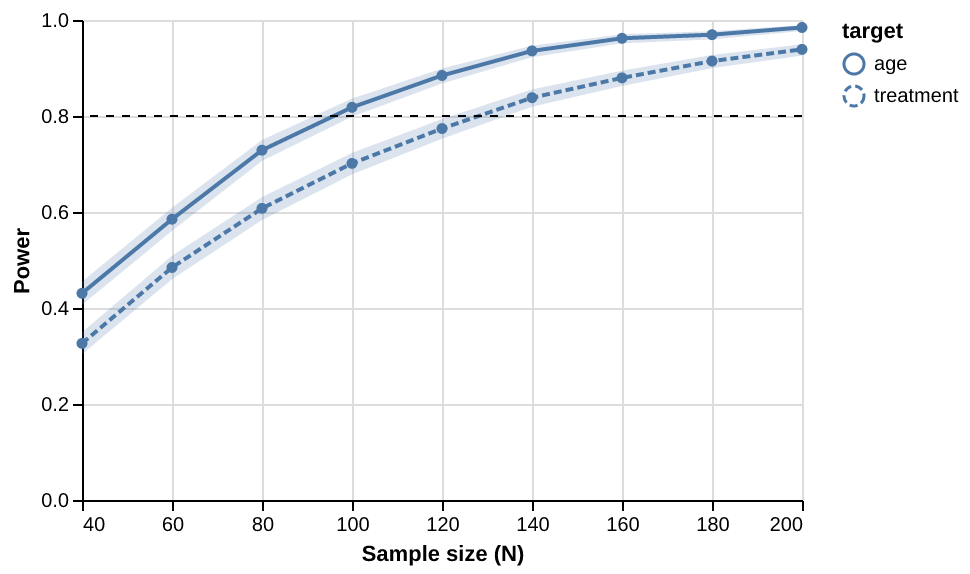
treatment needs N = 129, age 96 — note the answers land between grid points: the headline is read off the fitted power curve, not snapped to the nearest simulated size, and the Required N & 95% CI table puts a Monte-Carlo interval around each one. The joint detection rows are the figure to budget for: detecting both effects together needs N = 145, since a study is only as powered as its weakest planned test. The curve shows power climbing with sample size for each test. See how required N is estimated for the method and what the ≤ / ≥ / appr. markers mean when a search range misses the answer.

next → Interactions