Robustness & Custom Scenario Analysis in R
Every power number rests on a set of assumptions — specific effect sizes, a well-behaved residual structure, predictors drawn from the distributions you specified. Scenario analysis asks a harder question: if those assumptions are optimistic, how much do we lose?
MCPower answers it by re-running your analysis under alternative configurations called scenarios, adding a column per scenario to the power table so you can read robustness at a glance.
The built-in sweep
Pass scenarios = TRUE to activate the built-in three-scenario sweep —
optimistic, realistic, and doomer. The built-in profiles are
calibrated to represent a plausible range of real-world conditions without
requiring you to guess at parameter values:
Scenario analysis works for logistic models too —
the same call with family = "logit". See
Scenario analysis for which knobs apply per
model family. Mixed models do not support scenarios yet.
library(mcpower)

model <- MCPower$new("satisfaction ~ treatment + age")
model$set_variable_type("treatment=binary")
model$set_effects("treatment=0.5, age=0.3")

result <- model$find_power(sample_size = 150, target_test = "all", scenarios = TRUE, verbose = FALSE)
print(summary(result))
==================================================
  MCPower · Power Analysis
==================================================
formula: satisfaction ~ treatment + age
estimator: OLS  N=150  sims=1600  α=0.05  target=80%
effects: treatment=0.50, age=0.30

Per-test power
─────────────────────────────────────────────────────────────
Test                 optimistic   realistic   doomer   Target
─────────────────────────────────────────────────────────────
Overall F                 98.9%       97.6%    94.6%      80%
treatment                 86.4%       82.2%    76.4%      80%
age                       95.2%       90.2%    81.4%      80%
─────────────────────────────────────────────────────────────

Power & 95% CI — optimistic
───────────────────────────────────────────
Test                 Power           CI 95%
───────────────────────────────────────────
Overall F            98.9%   [98.2%, 99.3%]
treatment            86.4%   [84.6%, 88.0%]
age                  95.2%   [94.1%, 96.2%]
───────────────────────────────────────────
95% CIs are Monte-Carlo (Wilson), n_sims=1600.

Power & 95% CI — realistic
───────────────────────────────────────────
Test                 Power           CI 95%
───────────────────────────────────────────
Overall F            97.6%   [96.8%, 98.3%]
treatment            82.2%   [80.3%, 84.0%]
age                  90.2%   [88.7%, 91.6%]
───────────────────────────────────────────
95% CIs are Monte-Carlo (Wilson), n_sims=1600.

Power & 95% CI — doomer
───────────────────────────────────────────
Test                 Power           CI 95%
───────────────────────────────────────────
Overall F            94.6%   [93.3%, 95.6%]
treatment            76.4%   [74.3%, 78.5%]
age                  81.4%   [79.4%, 83.2%]
───────────────────────────────────────────
95% CIs are Monte-Carlo (Wilson), n_sims=1600.

Joint significance distribution
────────────────────────
k     Exactly   At least
────────────────────────
0        0.9%       100%
1       16.6%      99.1%
2       82.5%      82.5%
────────────────────────

Robustness  (Δ power vs baseline: optimistic)
─────────────────────────────────────────
Test                 realistic     doomer
─────────────────────────────────────────
treatment              -4.1 pp    -9.9 pp
age                    -5.0 pp   -13.9 pp
─────────────────────────────────────────

Plots: plot(result) to view, plot(result, 'chart.png') to save.
The power table gains three columns, one per scenario. Power erodes as
conditions worsen, and the two coefficients erode differently. age starts at
95.2% under optimistic conditions, eases to 90.2% under realistic, and falls to
81.4% under doomer; treatment slides from 86.4% to 82.2% to 76.4% — dipping
below the 80% target by the doomer scenario. The Robustness section at the
bottom makes the deltas explicit: by the doomer scenario age has lost 13.9
percentage points and treatment 9.9. age is the more sensitive to departures
from the idealised setup, but treatment — starting lower — is the one that
slips under target first.
The built-in sweep is a fast sanity check. If you need to represent domain-specific assumptions — e.g. a known degree of measurement noise or a near-certain distributional shift — use custom scenarios instead.
Custom scenario configs
model$set_scenario_configs accepts a named list of named lists. Each name is a
scenario name; each inner list is a set of knobs to override. The merge has
two branches: overriding a built-in name ("optimistic", "realistic",
"doomer") updates that preset — knobs you don't set keep their preset
values — while a brand-new name inherits all optimistic values and applies only
the overrides you give.
The available knobs are:
| Knob | What it perturbs |
|---|---|
heterogeneity |
The true effect varies from study to study — on average it's the effect you set, but any given simulation might draw 80% or 120% of it (SD = knob × effect). At large values this puts a hard cap on achievable power, no matter the sample size — see [[concepts/limitations |
heteroskedasticity_ratio |
Residual-variance ratio λ between high and low predicted values (1.0 = homoskedastic) |
correlation_noise_sd |
Jitter added to the predictor correlation structure |
distribution_change_prob |
Probability that a normal predictor is redrawn from a non-normal distribution |
residual_change_prob |
Probability that the residual distribution is swapped to a non-normal shape |
residual_dists |
Pool of replacement residual shapes: high_kurtosis (Student t, df from residual_df), right_skewed, left_skewed, normal, uniform |
residual_df |
Degrees of freedom for the replacement residual shapes (minimum 3) |
sampled_factor_proportions |
Factor group sizes: exact requested proportions when FALSE (the default), random per-observation assignment when TRUE |
Knob names are validated up front: an unknown or misspelled key raises an
error listing the valid keys, and arming the residual swap with a
high_kurtosis or right_skewed pool entry requires residual_df >= 3. See
Scenario analysis for every knob's full
semantics.
After registering configs, pass a character vector of names to scenarios to
choose which ones to run. Names that appear in the vector but have no registered
config are treated as aliases for the built-in profiles — so "optimistic" here
uses the built-in optimistic baseline:
library(mcpower)

model <- MCPower$new("satisfaction ~ treatment + age")
model$set_variable_type("treatment=binary")
model$set_effects("treatment=0.5, age=0.3")

model$set_scenario_configs(list(
  realistic   = list(heteroskedasticity_ratio = 3.0, correlation_noise_sd = 0.20),
  stress_test = list(heterogeneity = 0.5, heteroskedasticity_ratio = 5.0,
                     distribution_change_prob = 0.9)
))

result <- model$find_power(sample_size = 150, target_test = "all",
                           scenarios = c("optimistic", "realistic", "stress_test"), verbose = FALSE)
print(summary(result))
==================================================
  MCPower · Power Analysis
==================================================
formula: satisfaction ~ treatment + age
estimator: OLS  N=150  sims=1600  α=0.05  target=80%
effects: treatment=0.50, age=0.30

Per-test power
──────────────────────────────────────────────────────────────────
Test                 optimistic   realistic   stress_test   Target
──────────────────────────────────────────────────────────────────
Overall F                 98.9%       97.4%         93.0%      80%
treatment                 86.4%       82.2%         73.5%      80%
age                       95.2%       90.1%         78.2%      80%
──────────────────────────────────────────────────────────────────

Power & 95% CI — optimistic
───────────────────────────────────────────
Test                 Power           CI 95%
───────────────────────────────────────────
Overall F            98.9%   [98.2%, 99.3%]
treatment            86.4%   [84.6%, 88.0%]
age                  95.2%   [94.1%, 96.2%]
───────────────────────────────────────────
95% CIs are Monte-Carlo (Wilson), n_sims=1600.

Power & 95% CI — realistic
───────────────────────────────────────────
Test                 Power           CI 95%
───────────────────────────────────────────
Overall F            97.4%   [96.5%, 98.1%]
treatment            82.2%   [80.2%, 84.0%]
age                  90.1%   [88.5%, 91.4%]
───────────────────────────────────────────
95% CIs are Monte-Carlo (Wilson), n_sims=1600.

Power & 95% CI — stress_test
───────────────────────────────────────────
Test                 Power           CI 95%
───────────────────────────────────────────
Overall F            93.0%   [91.6%, 94.1%]
treatment            73.5%   [71.3%, 75.6%]
age                  78.2%   [76.2%, 80.2%]
───────────────────────────────────────────
95% CIs are Monte-Carlo (Wilson), n_sims=1600.

Joint significance distribution
────────────────────────
k     Exactly   At least
────────────────────────
0        0.9%       100%
1       16.6%      99.1%
2       82.5%      82.5%
────────────────────────

Robustness  (Δ power vs baseline: optimistic)
────────────────────────────────────────────
Test                 realistic   stress_test
────────────────────────────────────────────
treatment              -4.2 pp      -12.9 pp
age                    -5.2 pp      -17.0 pp
────────────────────────────────────────────

Plots: plot(result) to view, plot(result, 'chart.png') to save.
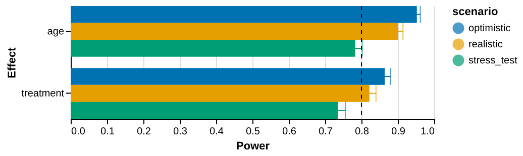
The chart below shows how power evolves across the three scenarios for each
test. Both coefficients slope downward as the knobs bite: age falls from
95.2% to 78.2% and treatment from 86.4% to 73.5% by the stress_test (high
heterogeneity, heavy heteroskedasticity, near-certain distributional shift),
which pushes both below the 80% target.
A brand-new scenario name (like stress_test) inherits the optimistic
baseline and applies only the keys you provide — omitted knobs stay at their
optimistic defaults. Overriding a built-in name (like realistic above)
instead updates that preset: omitted knobs keep their preset values.
Reading the output
Compare the 08-builtin and 08-custom results side by side. The realistic
column in both is nearly identical (~82% / ~90% for treatment/age) because
overriding a built-in name updates the preset: this custom realistic keeps
the realistic values for every knob it doesn't set and only raises
heteroskedasticity_ratio (2.0 → 3.0) and correlation_noise_sd (0.15 → 0.20).
The stress_test column replaces doomer and pushes harder on heterogeneity
and distribution_change_prob, landing near the doomer numbers for age (~80%
in both) while being explicitly designed around what you know about your domain.
That is the point of custom scenarios: you control what "pessimistic" means,
rather than accepting a one-size-fits-all profile.
next → Upload data