MCPower — Validating the Data Generator
What this report shows
MCPower answers power-analysis questions by generating synthetic
datasets from a formula you specify — for example “the outcome y
equals 0.25 × x1 plus random noise” — and then simulating your
analysis on those datasets many times. Everything downstream depends on
one thing being true: the data it generates must actually embody the
formula you asked for. If the generator is even slightly wrong, every
power number built on top of it is wrong too.
This report checks exactly that. For each supported formula we chose the true coefficients, so we know the right answer in advance. The question is simple:
When an independent, standard statistical analysis is run on MCPower’s generated data, does it recover the true numbers we put in?
If it does — consistently, across every supported kind of model — the generator is faithful.
How the data is generated
For each formula MCPower builds a dataset of n rows:
- continuous predictors are drawn from a standard normal distribution (average 0, standard deviation 1);
- categorical predictors (factors) are assigned at the requested proportions (a 2-level factor becomes a single 0/1 column; a 3-level factor becomes two);
- clustered (mixed-effects) data groups the rows and gives each group a shared random offset, sized to hit the requested intra-cluster correlation (ICC) — specifically the conditional ICC, the correlation that remains after the predictors are accounted for (the raw outcome’s marginal ICC is lower whenever the predictors explain variance);
- the outcome is computed from the true formula and coefficients, then random variation is added — standard-normal noise for ordinary regression, a 0/1 draw at the model’s probability for logistic regression, a cluster offset plus noise for mixed models.
A single dataset is noisy, so we never judge from one. Instead each formula is regenerated many times with fresh random noise — 1,600 times for ordinary and logistic models, 800 for mixed models — and we look at the distribution of results across all of those draws.
The three checks
1. Data checks. The basic statistics of the generated data should match what was requested: predictor averages near 0, standard deviations near 1, the requested correlations and factor proportions, the noise variance, and the ICC. We average each statistic over all draws (which cancels the random scatter of any single dataset) and require it to land within a small fixed tolerance of the requested value.
2. Coefficient recovery — the headline check: is the formula
actually true in the data? For every generated dataset we fit a
completely independent, standard model in R (lm, glm, or
lme4::lmer) and read off the estimated coefficients. Averaged over all
draws, each estimate should land on the true value we put in. We measure
how far the average estimate is from the truth in units of its own
standard error (the estimate’s draw-to-draw scatter divided by the
square root of the number of draws). For OLS and mixed-effects models,
the ~103 per-coefficient z-scores are pooled across all cases and the
false-discovery rate is controlled via Benjamini-Hochberg at q =
0.001 (a fixed per-coefficient z-threshold below ~4 would abort nearly
every clean render on sampling noise alone). For logistic regression we
use an absolute band instead (|mean − true| ≤ 0.02), because
logistic MLE’s finite-sample bias swamps the z-score at this K — see
below.
3. File reproduces. The dataset saved to disk for each formula is regenerated from its random seed, and its content fingerprint (a SHA-256 hash) is compared to the saved one. A mismatch would mean the generator’s output had drifted, so any later comparison against the saved file would be meaningless.
The thresholds
| What we check | Requested value | Allowed difference |
|---|---|---|
| average of each continuous predictor | 0 | within 0.01 |
| standard deviation of each predictor | 1 | within 0.01 |
| correlation between predictors | the value you set | within 0.01 |
| factor level proportions | the values you set | within 0.01 |
| noise / within-cluster variance | 1 | within 1% |
| intra-cluster correlation (ICC), conditional | the value you set | within 0.01 |
| observed (marginal) ICC vs predicted | τ²/(τ²+σ²+Var(Xβ)) | within 0.01 |
| coefficient recovery (OLS/LME) | the true coefficient | pooled BH-FDR ≤ 0.001 across all cases |
| coefficient recovery (logit) | the true coefficient | absolute difference within 0.02 |
The data-check tolerances are tight because they apply to the average over all draws, not to a single dataset — averaging thousands of draws removes the random scatter, so anything outside these bands signals a real generation problem.
A note on logistic regression. Logistic-regression estimates carry a small, well-known finite-sample bias: with a limited number of rows the maximum-likelihood estimate is slightly off even when everything is correct. With this many draws that tiny bias becomes statistically visible (the logistic models below show recovery distances running a bit higher, around 3–4 standard errors), but it stays within tolerance at the sample sizes used here. It is an expected statistical artefact, not a flaw in the generator.
Bias vs. spread. For each formula we report two different things separately. Bias is whether the average estimate is off the true value (a centring problem). Spread is how much the estimates vary from draw to draw. When two predictors are correlated, their estimates naturally vary more — collinearity inflates the spread. That wider spread is expected and correct; it is not a failure, and we say so wherever it appears.
Results at a glance
Every row is one formula with one set of true coefficients. “Data checks” and “Coefficient recovery” summarise the per-formula detail that follows.
| Formula | True coefficients | n | Data checks | Coefficient recovery | File reproduces |
|---|---|---|---|---|---|
y ~ x1 |
x1=0.25 |
400 | all OK | all OK | yes |
y ~ x1 |
x1=0.40 |
400 | all OK | all OK | yes |
y ~ x1 + x2 |
x1=0.25, x2=0.10 |
400 | all OK | all OK | yes |
y ~ x1 + x2 |
x1=0.40, x2=0.25 |
400 | all OK | all OK | yes |
y ~ x1 + x2 |
x1=0.25, x2=0.0 |
400 | all OK | all OK | yes |
y ~ x1 + x2 |
x1=0.25, x2=0.10 |
400 | all OK | all OK | yes |
y ~ x1 + x2 |
x1=0.40, x2=0.25 |
400 | all OK | all OK | yes |
y ~ x1*x2 |
x1=0.25, x2=0.10, x1:x2=-0.20 |
600 | all OK | all OK | yes |
y ~ x1*x2 |
x1=0.40, x2=0.25, x1:x2=0.15 |
600 | all OK | all OK | yes |
y ~ x1 + g |
x1=0.25, g[2]=0.50, g[3]=0.80 |
600 | all OK | all OK | yes |
y ~ x1 + g |
x1=0.40, g[2]=0.20, g[3]=0.50 |
600 | all OK | all OK | yes |
y ~ x1*g |
x1=0.30, g[2]=0.40, g[3]=0.60, x1:g[2]=0.20, x1:g[3]=0.30 |
800 | all OK | all OK | yes |
y ~ x1*g |
x1=0.40, g[2]=0.50, g[3]=0.80, x1:g[2]=0.25, x1:g[3]=0.40 |
800 | all OK | all OK | yes |
y ~ g1*g2 |
g1[2]=0.50, g2[2]=0.40, g1[2]:g2[2]=0.30 |
800 | all OK | all OK | yes |
y ~ g1*g2 |
g1[2]=0.20, g2[2]=0.80, g1[2]:g2[2]=0.50 |
800 | all OK | all OK | yes |
y ~ x1 |
x1=0.5 |
600 | all OK | all OK | yes |
y ~ x1 |
x1=0.8 |
600 | all OK | all OK | yes |
y ~ x1 + x2 |
x1=0.5, x2=0.3 |
800 | all OK | all OK | yes |
y ~ x1 + x2 |
x1=0.8, x2=0.5 |
800 | all OK | all OK | yes |
y ~ x1 + g |
x1=0.5, g[2]=0.4, g[3]=0.8 |
1000 | all OK | all OK | yes |
y ~ x1 + g |
x1=0.8, g[2]=0.5, g[3]=0.8 |
1000 | all OK | all OK | yes |
y ~ x1*x2 |
x1=0.5, x2=0.3, x1:x2=0.3 |
1000 | all OK | all OK | yes |
y ~ x1*x2 |
x1=0.8, x2=0.5, x1:x2=0.4 |
1000 | all OK | all OK | yes |
y ~ x1 + (1|grp) |
x1=0.5 |
600 | all OK | all OK | yes |
y ~ x1 + (1|grp) |
x1=0.3 |
600 | all OK | all OK | yes |
y ~ x1 + x2 + (1|grp) |
x1=0.5, x2=0.3 |
750 | all OK | all OK | yes |
y ~ x1 + x2 + (1|grp) |
x1=0.3, x2=0.5 |
750 | all OK | all OK | yes |
y ~ x1*x2 + (1|grp) |
x1=0.5, x2=0.3, x1:x2=0.3 |
750 | all OK | all OK | yes |
y ~ x1*x2 + (1|grp) |
x1=0.4, x2=0.3, x1:x2=0.2 |
900 | all OK | all OK | yes |
y ~ x1 + g + (1|grp) |
x1=0.30, g[2]=0.30 |
750 | all OK | all OK | yes |
y ~ x1 + g + (1|grp) |
x1=0.40, g[2]=0.50, g[3]=0.80 |
900 | all OK | all OK | yes |
All 31 formulas pass all three checks. The generated data matches the requested statistics, an independent R model recovers every true coefficient, and every saved dataset reproduces from its seed.
Formula-by-formula detail
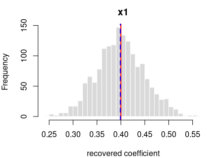
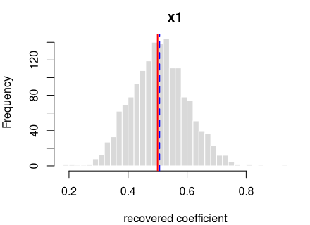
y = 0.25·x1 + noise
R formula y ~ x1 · ordinary least squares (R’s lm) · n = 400 · saved
as data/ols_simple_a.rds
How it’s built: one continuous predictor (x1) drawn from a
standard normal (mean 0, sd 1). The outcome is the formula above plus
standard-normal noise. Sample size 400, random seed 2137.
Data checks — statistics of the generated data, averaged over all draws, vs. what was requested:
| What we check | Requested | Average over draws | Allowed difference | Result |
|---|---|---|---|---|
| average of x1 | 0 | 0.0003 | within 0.01 | OK |
| std. deviation of x1 | 1 | 0.9999 | within 0.01 | OK |
| noise variance | 1 | 0.9987 | within 1% | OK |
Coefficient recovery — an independent R model fitted to each generated dataset; the average estimate should land on the true value:
| Term | True value | Recovered (average) | Spread across draws | Std. errors from true | Result |
|---|---|---|---|---|---|
| intercept | 0.00 | 0.0009 | 0.0503 | 0.7213 | OK |
| x1 | 0.25 | 0.2490 | 0.0499 | -0.8197 | OK |
Every coefficient is centred on its true value — the formula holds in the generated data.

Each panel: the spread of one recovered coefficient across 1600 generated datasets. Red line = the true value, blue dashed = the average estimate. File reproduces from seed: yes.
y = 0.4·x1 + noise
R formula y ~ x1 · ordinary least squares (R’s lm) · n = 400 · saved
as data/ols_simple_b.rds
How it’s built: one continuous predictor (x1) drawn from a
standard normal (mean 0, sd 1). The outcome is the formula above plus
standard-normal noise. Sample size 400, random seed 2138.
Data checks — statistics of the generated data, averaged over all draws, vs. what was requested:
| What we check | Requested | Average over draws | Allowed difference | Result |
|---|---|---|---|---|
| average of x1 | 0 | 0.0003 | within 0.01 | OK |
| std. deviation of x1 | 1 | 0.9999 | within 0.01 | OK |
| noise variance | 1 | 0.9986 | within 1% | OK |
Coefficient recovery — an independent R model fitted to each generated dataset; the average estimate should land on the true value:
| Term | True value | Recovered (average) | Spread across draws | Std. errors from true | Result |
|---|---|---|---|---|---|
| intercept | 0.0 | 0.0009 | 0.0503 | 0.7157 | OK |
| x1 | 0.4 | 0.3989 | 0.0499 | -0.8420 | OK |
Every coefficient is centred on its true value — the formula holds in the generated data.
Each panel: the spread of one recovered coefficient across 1600 generated datasets. Red line = the true value, blue dashed = the average estimate. File reproduces from seed: yes.
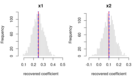
y = 0.25·x1 + 0.1·x2 + noise
R formula y ~ x1 + x2 · ordinary least squares (R’s lm) · n = 400 ·
saved as data/ols_two_a.rds
How it’s built: 2 continuous predictors (x1, x2) drawn from a
standard normal (mean 0, sd 1). The outcome is the formula above plus
standard-normal noise. Sample size 400, random seed 2137.
Data checks — statistics of the generated data, averaged over all draws, vs. what was requested:
| What we check | Requested | Average over draws | Allowed difference | Result |
|---|---|---|---|---|
| average of x1 | 0 | 0.0003 | within 0.01 | OK |
| std. deviation of x1 | 1 | 0.9999 | within 0.01 | OK |
| average of x2 | 0 | 0.0016 | within 0.01 | OK |
| std. deviation of x2 | 1 | 0.9987 | within 0.01 | OK |
| noise variance | 1 | 0.9986 | within 1% | OK |
Coefficient recovery — an independent R model fitted to each generated dataset; the average estimate should land on the true value:
| Term | True value | Recovered (average) | Spread across draws | Std. errors from true | Result |
|---|---|---|---|---|---|
| intercept | 0.00 | 0.0009 | 0.0504 | 0.7429 | OK |
| x1 | 0.25 | 0.2490 | 0.0500 | -0.8043 | OK |
| x2 | 0.10 | 0.1018 | 0.0512 | 1.4445 | OK |
Every coefficient is centred on its true value — the formula holds in the generated data.
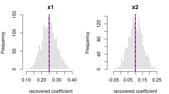
Each panel: the spread of one recovered coefficient across 1600 generated datasets. Red line = the true value, blue dashed = the average estimate. File reproduces from seed: yes.
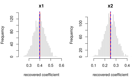
y = 0.4·x1 + 0.25·x2 + noise
R formula y ~ x1 + x2 · ordinary least squares (R’s lm) · n = 400 ·
saved as data/ols_two_b.rds
How it’s built: 2 continuous predictors (x1, x2) drawn from a
standard normal (mean 0, sd 1). The outcome is the formula above plus
standard-normal noise. Sample size 400, random seed 2138.
Data checks — statistics of the generated data, averaged over all draws, vs. what was requested:
| What we check | Requested | Average over draws | Allowed difference | Result |
|---|---|---|---|---|
| average of x1 | 0 | 0.0003 | within 0.01 | OK |
| std. deviation of x1 | 1 | 0.9999 | within 0.01 | OK |
| average of x2 | 0 | 0.0016 | within 0.01 | OK |
| std. deviation of x2 | 1 | 0.9987 | within 0.01 | OK |
| noise variance | 1 | 0.9985 | within 1% | OK |
Coefficient recovery — an independent R model fitted to each generated dataset; the average estimate should land on the true value:
| Term | True value | Recovered (average) | Spread across draws | Std. errors from true | Result |
|---|---|---|---|---|---|
| intercept | 0.00 | 0.0009 | 0.0504 | 0.7352 | OK |
| x1 | 0.40 | 0.3990 | 0.0499 | -0.8285 | OK |
| x2 | 0.25 | 0.2519 | 0.0512 | 1.4579 | OK |
Every coefficient is centred on its true value — the formula holds in the generated data.
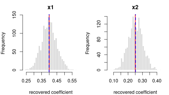
Each panel: the spread of one recovered coefficient across 1600 generated datasets. Red line = the true value, blue dashed = the average estimate. File reproduces from seed: yes.
y = 0.25·x1 + 0·x2 + noise
R formula y ~ x1 + x2 · ordinary least squares (R’s lm) · n = 400 ·
saved as data/ols_zero_a.rds
How it’s built: 2 continuous predictors (x1, x2) drawn from a
standard normal (mean 0, sd 1). The outcome is the formula above plus
standard-normal noise. Sample size 400, random seed 2137.
Data checks — statistics of the generated data, averaged over all draws, vs. what was requested:
| What we check | Requested | Average over draws | Allowed difference | Result |
|---|---|---|---|---|
| average of x1 | 0 | 0.0003 | within 0.01 | OK |
| std. deviation of x1 | 1 | 0.9999 | within 0.01 | OK |
| average of x2 | 0 | 0.0016 | within 0.01 | OK |
| std. deviation of x2 | 1 | 0.9987 | within 0.01 | OK |
| noise variance | 1 | 0.9986 | within 1% | OK |
Coefficient recovery — an independent R model fitted to each generated dataset; the average estimate should land on the true value:
| Term | True value | Recovered (average) | Spread across draws | Std. errors from true | Result |
|---|---|---|---|---|---|
| intercept | 0.00 | 0.0009 | 0.0504 | 0.7429 | OK |
| x1 | 0.25 | 0.2490 | 0.0500 | -0.8043 | OK |
| x2 | 0.00 | 0.0018 | 0.0512 | 1.4445 | OK |
Every coefficient is centred on its true value — the formula holds in the generated data.
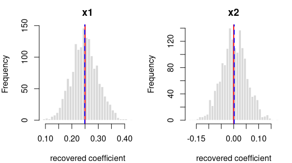
Each panel: the spread of one recovered coefficient across 1600 generated datasets. Red line = the true value, blue dashed = the average estimate. File reproduces from seed: yes.
y = 0.25·x1 + 0.1·x2 + noise
R formula y ~ x1 + x2 · ordinary least squares (R’s lm) · n = 400 ·
saved as data/ols_corr_a.rds
How it’s built: 2 continuous predictors (x1, x2) drawn from a
standard normal (mean 0, sd 1); x1 and x2 correlated at 0.50. The
outcome is the formula above plus standard-normal noise. Sample size
400, random seed 2137.
Data checks — statistics of the generated data, averaged over all draws, vs. what was requested:
| What we check | Requested | Average over draws | Allowed difference | Result |
|---|---|---|---|---|
| average of x1 | 0.0 | 0.0003 | within 0.01 | OK |
| std. deviation of x1 | 1.0 | 0.9999 | within 0.01 | OK |
| average of x2 | 0.0 | 0.0015 | within 0.01 | OK |
| std. deviation of x2 | 1.0 | 0.9988 | within 0.01 | OK |
| correlation of x1 and x2 | 0.5 | 0.4997 | within 0.01 | OK |
| noise variance | 1.0 | 0.9986 | within 1% | OK |
Coefficient recovery — an independent R model fitted to each generated dataset; the average estimate should land on the true value:
| Term | True value | Recovered (average) | Spread across draws | Std. errors from true | Result |
|---|---|---|---|---|---|
| intercept | 0.00 | 0.0009 | 0.0504 | 0.7429 | OK |
| x1 | 0.25 | 0.2479 | 0.0575 | -1.4427 | OK |
| x2 | 0.10 | 0.1021 | 0.0591 | 1.4445 | OK |
Every coefficient is centred on its true value — the formula holds in
the generated data. Because x1 and x2 are correlated (0.50), their
estimates vary more from draw to draw; that wider spread is the expected
effect of collinearity, not a problem.
Each panel: the spread of one recovered coefficient across 1600 generated datasets. Red line = the true value, blue dashed = the average estimate. File reproduces from seed: yes.
y = 0.4·x1 + 0.25·x2 + noise
R formula y ~ x1 + x2 · ordinary least squares (R’s lm) · n = 400 ·
saved as data/ols_corr_b.rds
How it’s built: 2 continuous predictors (x1, x2) drawn from a
standard normal (mean 0, sd 1); x1 and x2 correlated at 0.30. The
outcome is the formula above plus standard-normal noise. Sample size
400, random seed 2138.
Data checks — statistics of the generated data, averaged over all draws, vs. what was requested:
| What we check | Requested | Average over draws | Allowed difference | Result |
|---|---|---|---|---|
| average of x1 | 0.0 | 0.0003 | within 0.01 | OK |
| std. deviation of x1 | 1.0 | 0.9999 | within 0.01 | OK |
| average of x2 | 0.0 | 0.0016 | within 0.01 | OK |
| std. deviation of x2 | 1.0 | 0.9987 | within 0.01 | OK |
| correlation of x1 and x2 | 0.3 | 0.2997 | within 0.01 | OK |
| noise variance | 1.0 | 0.9985 | within 1% | OK |
Coefficient recovery — an independent R model fitted to each generated dataset; the average estimate should land on the true value:
| Term | True value | Recovered (average) | Spread across draws | Std. errors from true | Result |
|---|---|---|---|---|---|
| intercept | 0.00 | 0.0009 | 0.0504 | 0.7352 | OK |
| x1 | 0.40 | 0.3984 | 0.0521 | -1.2446 | OK |
| x2 | 0.25 | 0.2520 | 0.0537 | 1.4579 | OK |
Every coefficient is centred on its true value — the formula holds in
the generated data. Because x1 and x2 are correlated (0.30), their
estimates vary more from draw to draw; that wider spread is the expected
effect of collinearity, not a problem.
Each panel: the spread of one recovered coefficient across 1600 generated datasets. Red line = the true value, blue dashed = the average estimate. File reproduces from seed: yes.
y = 0.25·x1 + 0.1·x2 − 0.2·x1:x2 + noise
R formula y ~ x1*x2 · ordinary least squares (R’s lm) · n = 600 ·
saved as data/ols_interaction_a.rds
How it’s built: 2 continuous predictors (x1, x2) drawn from a
standard normal (mean 0, sd 1); x1 and x2 correlated at 0.30. The
outcome is the formula above plus standard-normal noise. Sample size
600, random seed 2137.
Data checks — statistics of the generated data, averaged over all draws, vs. what was requested:
| What we check | Requested | Average over draws | Allowed difference | Result |
|---|---|---|---|---|
| average of x1 | 0.0 | 0.0002 | within 0.01 | OK |
| std. deviation of x1 | 1.0 | 0.9998 | within 0.01 | OK |
| average of x2 | 0.0 | 0.0012 | within 0.01 | OK |
| std. deviation of x2 | 1.0 | 0.9994 | within 0.01 | OK |
| correlation of x1 and x2 | 0.3 | 0.3000 | within 0.01 | OK |
| noise variance | 1.0 | 1.0006 | within 1% | OK |
Coefficient recovery — an independent R model fitted to each generated dataset; the average estimate should land on the true value:
| Term | True value | Recovered (average) | Spread across draws | Std. errors from true | Result |
|---|---|---|---|---|---|
| intercept | 0.00 | 0.0024 | 0.0420 | 2.3300 | OK |
| x1 | 0.25 | 0.2479 | 0.0421 | -1.9544 | OK |
| x2 | 0.10 | 0.1018 | 0.0437 | 1.6031 | OK |
| x1:x2 | -0.20 | -0.2002 | 0.0386 | -0.1597 | OK |
Every coefficient is centred on its true value — the formula holds in
the generated data. Because x1 and x2 are correlated (0.30), their
estimates vary more from draw to draw; that wider spread is the expected
effect of collinearity, not a problem.
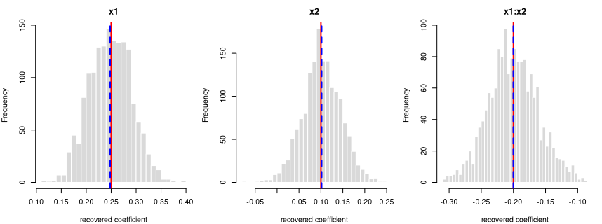
Each panel: the spread of one recovered coefficient across 1600 generated datasets. Red line = the true value, blue dashed = the average estimate. File reproduces from seed: yes.
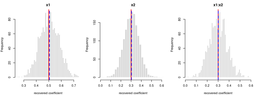
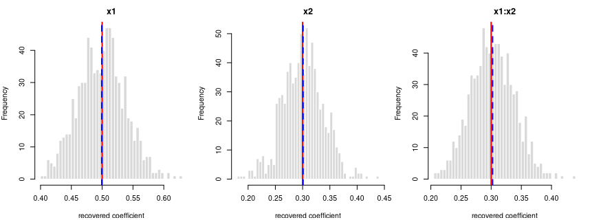
y = 0.4·x1 + 0.25·x2 + 0.15·x1:x2 + noise
R formula y ~ x1*x2 · ordinary least squares (R’s lm) · n = 600 ·
saved as data/ols_interaction_b.rds
How it’s built: 2 continuous predictors (x1, x2) drawn from a
standard normal (mean 0, sd 1). The outcome is the formula above plus
standard-normal noise. Sample size 600, random seed 2138.
Data checks — statistics of the generated data, averaged over all draws, vs. what was requested:
| What we check | Requested | Average over draws | Allowed difference | Result |
|---|---|---|---|---|
| average of x1 | 0 | 0.0002 | within 0.01 | OK |
| std. deviation of x1 | 1 | 0.9998 | within 0.01 | OK |
| average of x2 | 0 | 0.0012 | within 0.01 | OK |
| std. deviation of x2 | 1 | 0.9993 | within 0.01 | OK |
| noise variance | 1 | 1.0006 | within 1% | OK |
Coefficient recovery — an independent R model fitted to each generated dataset; the average estimate should land on the true value:
| Term | True value | Recovered (average) | Spread across draws | Std. errors from true | Result |
|---|---|---|---|---|---|
| intercept | 0.00 | 0.0024 | 0.0404 | 2.3519 | OK |
| x1 | 0.40 | 0.3984 | 0.0404 | -1.5424 | OK |
| x2 | 0.25 | 0.2517 | 0.0418 | 1.5936 | OK |
| x1:x2 | 0.15 | 0.1500 | 0.0400 | -0.0045 | OK |
Every coefficient is centred on its true value — the formula holds in the generated data.
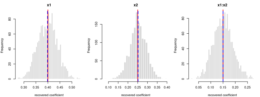
Each panel: the spread of one recovered coefficient across 1600 generated datasets. Red line = the true value, blue dashed = the average estimate. File reproduces from seed: yes.
y = 0.25·x1 + 0.5·g[2] + 0.8·g[3] + noise
R formula y ~ x1 + g · ordinary least squares (R’s lm) · n = 600 ·
saved as data/ols_factor_a.rds
How it’s built: one continuous predictor (x1) drawn from a
standard normal (mean 0, sd 1); a 3-level factor g at proportions
50%/30%/20%. The outcome is the formula above plus standard-normal
noise. Sample size 600, random seed 2137.
Data checks — statistics of the generated data, averaged over all draws, vs. what was requested:
| What we check | Requested | Average over draws | Allowed difference | Result |
|---|---|---|---|---|
| average of x1 | 0.0 | 0.0002 | within 0.01 | OK |
| std. deviation of x1 | 1.0 | 0.9998 | within 0.01 | OK |
| proportion in level 0 | 0.5 | 0.5000 | within 0.01 | OK |
| proportion in level 1 | 0.3 | 0.3000 | within 0.01 | OK |
| proportion in level 2 | 0.2 | 0.2000 | within 0.01 | OK |
| noise variance | 1.0 | 1.0006 | within 1% | OK |
Coefficient recovery — an independent R model fitted to each generated dataset; the average estimate should land on the true value:
| Term | True value | Recovered (average) | Spread across draws | Std. errors from true | Result |
|---|---|---|---|---|---|
| intercept | 0.00 | 0.0019 | 0.0575 | 1.3304 | OK |
| x1 | 0.25 | 0.2484 | 0.0404 | -1.5703 | OK |
| g[2] | 0.50 | 0.5006 | 0.0940 | 0.2410 | OK |
| g[3] | 0.80 | 0.8017 | 0.1081 | 0.6291 | OK |
Every coefficient is centred on its true value — the formula holds in the generated data.
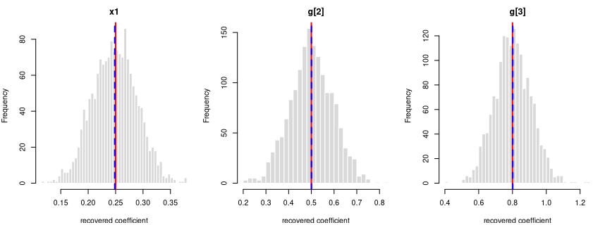
Each panel: the spread of one recovered coefficient across 1600 generated datasets. Red line = the true value, blue dashed = the average estimate. File reproduces from seed: yes.
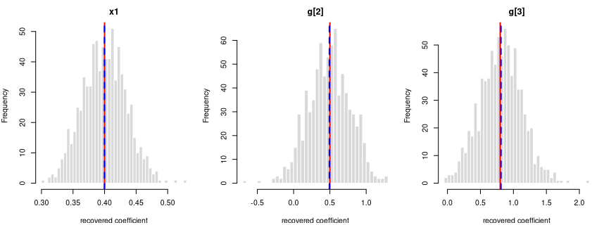
y = 0.4·x1 + 0.2·g[2] + 0.5·g[3] + noise
R formula y ~ x1 + g · ordinary least squares (R’s lm) · n = 600 ·
saved as data/ols_factor_b.rds
How it’s built: one continuous predictor (x1) drawn from a
standard normal (mean 0, sd 1); a 3-level factor g at proportions
40%/35%/25%. The outcome is the formula above plus standard-normal
noise. Sample size 600, random seed 2138.
Data checks — statistics of the generated data, averaged over all draws, vs. what was requested:
| What we check | Requested | Average over draws | Allowed difference | Result |
|---|---|---|---|---|
| average of x1 | 0.00 | 0.0002 | within 0.01 | OK |
| std. deviation of x1 | 1.00 | 0.9998 | within 0.01 | OK |
| proportion in level 0 | 0.40 | 0.4000 | within 0.01 | OK |
| proportion in level 1 | 0.35 | 0.3500 | within 0.01 | OK |
| proportion in level 2 | 0.25 | 0.2500 | within 0.01 | OK |
| noise variance | 1.00 | 1.0006 | within 1% | OK |
Coefficient recovery — an independent R model fitted to each generated dataset; the average estimate should land on the true value:
| Term | True value | Recovered (average) | Spread across draws | Std. errors from true | Result |
|---|---|---|---|---|---|
| intercept | 0.0 | 0.0014 | 0.0640 | 0.8709 | OK |
| x1 | 0.4 | 0.3984 | 0.0405 | -1.6196 | OK |
| g[2] | 0.2 | 0.2030 | 0.0938 | 1.2617 | OK |
| g[3] | 0.5 | 0.4999 | 0.1034 | -0.0267 | OK |
Every coefficient is centred on its true value — the formula holds in the generated data.
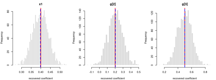
Each panel: the spread of one recovered coefficient across 1600 generated datasets. Red line = the true value, blue dashed = the average estimate. File reproduces from seed: yes.
y = 0.3·x1 + 0.4·g[2] + 0.6·g[3] + 0.2·x1:g[2] + 0.3·x1:g[3] + noise
R formula y ~ x1*g · ordinary least squares (R’s lm) · n = 800 ·
saved as data/ols_cf_a.rds
How it’s built: one continuous predictor (x1) drawn from a
standard normal (mean 0, sd 1); a 3-level factor g at proportions
50%/30%/20%. The outcome is the formula above plus standard-normal
noise. Sample size 800, random seed 2137.
Data checks — statistics of the generated data, averaged over all draws, vs. what was requested:
| What we check | Requested | Average over draws | Allowed difference | Result |
|---|---|---|---|---|
| average of x1 | 0.0 | 0.0014 | within 0.01 | OK |
| std. deviation of x1 | 1.0 | 1.0000 | within 0.01 | OK |
| proportion in level 0 | 0.5 | 0.5000 | within 0.01 | OK |
| proportion in level 1 | 0.3 | 0.3000 | within 0.01 | OK |
| proportion in level 2 | 0.2 | 0.2000 | within 0.01 | OK |
| noise variance | 1.0 | 1.0007 | within 1% | OK |
Coefficient recovery — an independent R model fitted to each generated dataset; the average estimate should land on the true value:
| Term | True value | Recovered (average) | Spread across draws | Std. errors from true | Result |
|---|---|---|---|---|---|
| intercept | 0.0 | 0.0008 | 0.0506 | 0.6615 | OK |
| x1 | 0.3 | 0.2974 | 0.0502 | -2.0526 | OK |
| g[2] | 0.4 | 0.4013 | 0.0826 | 0.6342 | OK |
| g[3] | 0.6 | 0.6013 | 0.0946 | 0.5694 | OK |
| x1:g[2] | 0.2 | 0.2014 | 0.0812 | 0.6654 | OK |
| x1:g[3] | 0.3 | 0.3056 | 0.0972 | 2.3123 | OK |
Every coefficient is centred on its true value — the formula holds in the generated data.
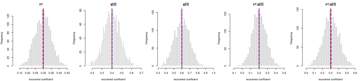
Each panel: the spread of one recovered coefficient across 1600 generated datasets. Red line = the true value, blue dashed = the average estimate. File reproduces from seed: yes.
y = 0.4·x1 + 0.5·g[2] + 0.8·g[3] + 0.25·x1:g[2] + 0.4·x1:g[3] + noise
R formula y ~ x1*g · ordinary least squares (R’s lm) · n = 800 ·
saved as data/ols_cf_b.rds
How it’s built: one continuous predictor (x1) drawn from a
standard normal (mean 0, sd 1); a 3-level factor g at proportions
40%/35%/25%. The outcome is the formula above plus standard-normal
noise. Sample size 800, random seed 2138.
Data checks — statistics of the generated data, averaged over all draws, vs. what was requested:
| What we check | Requested | Average over draws | Allowed difference | Result |
|---|---|---|---|---|
| average of x1 | 0.00 | 0.0014 | within 0.01 | OK |
| std. deviation of x1 | 1.00 | 1.0000 | within 0.01 | OK |
| proportion in level 0 | 0.40 | 0.4000 | within 0.01 | OK |
| proportion in level 1 | 0.35 | 0.3500 | within 0.01 | OK |
| proportion in level 2 | 0.25 | 0.2500 | within 0.01 | OK |
| noise variance | 1.00 | 1.0006 | within 1% | OK |
Coefficient recovery — an independent R model fitted to each generated dataset; the average estimate should land on the true value:
| Term | True value | Recovered (average) | Spread across draws | Std. errors from true | Result |
|---|---|---|---|---|---|
| intercept | 0.00 | 0.0013 | 0.0554 | 0.9654 | OK |
| x1 | 0.40 | 0.3963 | 0.0577 | -2.5524 | OK |
| g[2] | 0.50 | 0.5015 | 0.0826 | 0.7481 | OK |
| g[3] | 0.80 | 0.7988 | 0.0904 | -0.5218 | OK |
| x1:g[2] | 0.25 | 0.2528 | 0.0839 | 1.3386 | OK |
| x1:g[3] | 0.40 | 0.4061 | 0.0916 | 2.6768 | OK |
Every coefficient is centred on its true value — the formula holds in the generated data.
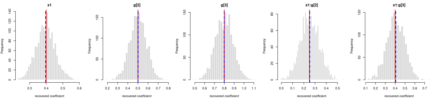
Each panel: the spread of one recovered coefficient across 1600 generated datasets. Red line = the true value, blue dashed = the average estimate. File reproduces from seed: yes.
y = 0.5·g1[2] + 0.4·g2[2] + 0.3·g1[2]:g2[2] + noise
R formula y ~ g1*g2 · ordinary least squares (R’s lm) · n = 800 ·
saved as data/ols_ff_a.rds
How it’s built: a 2-level factor g1 at proportions 50%/50%; a
2-level factor g2 at proportions 60%/40%. The outcome is the formula
above plus standard-normal noise. Sample size 800, random seed 2137.
Data checks — statistics of the generated data, averaged over all draws, vs. what was requested:
| What we check | Requested | Average over draws | Allowed difference | Result |
|---|---|---|---|---|
| noise variance | 1 | 1.0007 | within 1% | OK |
Coefficient recovery — an independent R model fitted to each generated dataset; the average estimate should land on the true value:
| Term | True value | Recovered (average) | Spread across draws | Std. errors from true | Result |
|---|---|---|---|---|---|
| intercept | 0.0 | 0.0000 | 0.0619 | 0.0222 | OK |
| g1[2] | 0.5 | 0.5025 | 0.0888 | 1.1111 | OK |
| g2[2] | 0.4 | 0.3992 | 0.0992 | -0.3184 | OK |
| g1[2]:g2[2] | 0.3 | 0.3030 | 0.1451 | 0.8201 | OK |
Every coefficient is centred on its true value — the formula holds in the generated data.
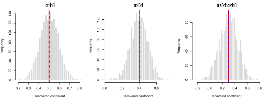
Each panel: the spread of one recovered coefficient across 1600 generated datasets. Red line = the true value, blue dashed = the average estimate. File reproduces from seed: yes.
y = 0.2·g1[2] + 0.8·g2[2] + 0.5·g1[2]:g2[2] + noise
R formula y ~ g1*g2 · ordinary least squares (R’s lm) · n = 800 ·
saved as data/ols_ff_b.rds
How it’s built: a 2-level factor g1 at proportions 50%/50%; a
2-level factor g2 at proportions 55%/45%. The outcome is the formula
above plus standard-normal noise. Sample size 800, random seed 2138.
Data checks — statistics of the generated data, averaged over all draws, vs. what was requested:
| What we check | Requested | Average over draws | Allowed difference | Result |
|---|---|---|---|---|
| noise variance | 1 | 1.0007 | within 1% | OK |
Coefficient recovery — an independent R model fitted to each generated dataset; the average estimate should land on the true value:
| Term | True value | Recovered (average) | Spread across draws | Std. errors from true | Result |
|---|---|---|---|---|---|
| intercept | 0.0 | -0.0005 | 0.0701 | -0.2752 | OK |
| g1[2] | 0.2 | 0.2026 | 0.0968 | 1.0546 | OK |
| g2[2] | 0.8 | 0.8004 | 0.0988 | 0.1608 | OK |
| g1[2]:g2[2] | 0.5 | 0.5028 | 0.1490 | 0.7572 | OK |
Every coefficient is centred on its true value — the formula holds in the generated data.
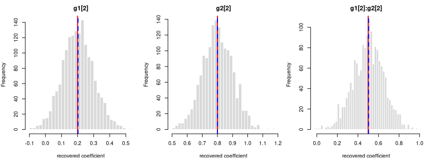
Each panel: the spread of one recovered coefficient across 1600 generated datasets. Red line = the true value, blue dashed = the average estimate. File reproduces from seed: yes.
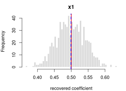
log-odds(y = 1) = logit(0.30) + 0.5·x1
R formula y ~ x1 · logistic regression (R’s glm) · n = 600 · saved
as data/glm_simple_a.rds
How it’s built: one continuous predictor (x1) drawn from a
standard normal (mean 0, sd 1). The outcome is 1 or 0, drawn at the
logistic probability of the formula above (baseline rate 30%). Sample
size 600, random seed 2137.
Data checks — statistics of the generated data, averaged over all draws, vs. what was requested:
| What we check | Requested | Average over draws | Allowed difference | Result |
|---|---|---|---|---|
| average of x1 | 0 | 0.0002 | within 0.01 | OK |
| std. deviation of x1 | 1 | 0.9998 | within 0.01 | OK |
Coefficient recovery — an independent R model fitted to each generated dataset; the average estimate should land on the true value:
| Term | True value | Recovered (average) | Spread across draws | Std. errors from true | Result |
|---|---|---|---|---|---|
| intercept | -0.8473 | -0.8543 | 0.0931 | -2.9921 | OK |
| x1 | 0.5000 | 0.5063 | 0.0951 | 2.6404 | OK |
Every coefficient is centred on its true value — the formula holds in the generated data.
Each panel: the spread of one recovered coefficient across 1600 generated datasets. Red line = the true value, blue dashed = the average estimate. File reproduces from seed: yes.
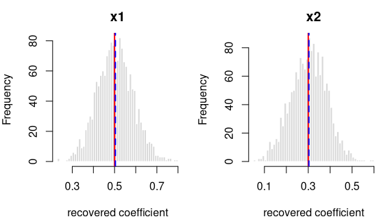
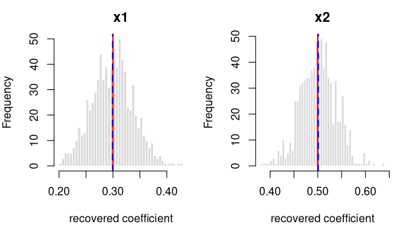
log-odds(y = 1) = logit(0.50) + 0.8·x1
R formula y ~ x1 · logistic regression (R’s glm) · n = 600 · saved
as data/glm_simple_b.rds
How it’s built: one continuous predictor (x1) drawn from a
standard normal (mean 0, sd 1). The outcome is 1 or 0, drawn at the
logistic probability of the formula above (baseline rate 50%). Sample
size 600, random seed 2138.
Data checks — statistics of the generated data, averaged over all draws, vs. what was requested:
| What we check | Requested | Average over draws | Allowed difference | Result |
|---|---|---|---|---|
| average of x1 | 0 | 0.0002 | within 0.01 | OK |
| std. deviation of x1 | 1 | 0.9998 | within 0.01 | OK |
Coefficient recovery — an independent R model fitted to each generated dataset; the average estimate should land on the true value:
| Term | True value | Recovered (average) | Spread across draws | Std. errors from true | Result |
|---|---|---|---|---|---|
| intercept | 0.0 | -0.0038 | 0.0858 | -1.7599 | OK |
| x1 | 0.8 | 0.8109 | 0.1025 | 4.2568 | OK |
Every coefficient is centred on its true value — the formula holds in the generated data.
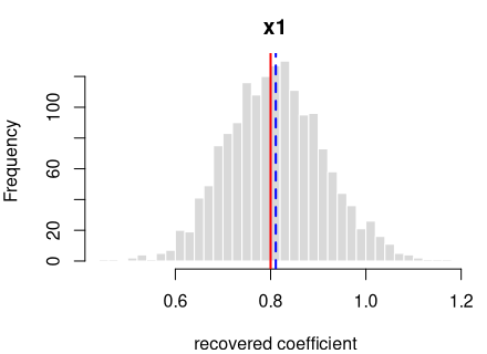
Each panel: the spread of one recovered coefficient across 1600 generated datasets. Red line = the true value, blue dashed = the average estimate. File reproduces from seed: yes.
log-odds(y = 1) = logit(0.30) + 0.5·x1 + 0.3·x2
R formula y ~ x1 + x2 · logistic regression (R’s glm) · n = 800 ·
saved as data/glm_two_a.rds
How it’s built: 2 continuous predictors (x1, x2) drawn from a
standard normal (mean 0, sd 1); x1 and x2 correlated at 0.20. The
outcome is 1 or 0, drawn at the logistic probability of the formula
above (baseline rate 30%). Sample size 800, random seed 2137.
Data checks — statistics of the generated data, averaged over all draws, vs. what was requested:
| What we check | Requested | Average over draws | Allowed difference | Result |
|---|---|---|---|---|
| average of x1 | 0.0 | 0.0014 | within 0.01 | OK |
| std. deviation of x1 | 1.0 | 1.0000 | within 0.01 | OK |
| average of x2 | 0.0 | 0.0010 | within 0.01 | OK |
| std. deviation of x2 | 1.0 | 0.9995 | within 0.01 | OK |
| correlation of x1 and x2 | 0.2 | 0.2001 | within 0.01 | OK |
Coefficient recovery — an independent R model fitted to each generated dataset; the average estimate should land on the true value:
| Term | True value | Recovered (average) | Spread across draws | Std. errors from true | Result |
|---|---|---|---|---|---|
| intercept | -0.8473 | -0.8528 | 0.0810 | -2.7143 | OK |
| x1 | 0.5000 | 0.5037 | 0.0852 | 1.7568 | OK |
| x2 | 0.3000 | 0.3028 | 0.0813 | 1.3693 | OK |
Every coefficient is centred on its true value — the formula holds in
the generated data. Because x1 and x2 are correlated (0.20), their
estimates vary more from draw to draw; that wider spread is the expected
effect of collinearity, not a problem.
Each panel: the spread of one recovered coefficient across 1600 generated datasets. Red line = the true value, blue dashed = the average estimate. File reproduces from seed: yes.
log-odds(y = 1) = logit(0.50) + 0.8·x1 + 0.5·x2
R formula y ~ x1 + x2 · logistic regression (R’s glm) · n = 800 ·
saved as data/glm_two_b.rds
How it’s built: 2 continuous predictors (x1, x2) drawn from a
standard normal (mean 0, sd 1). The outcome is 1 or 0, drawn at the
logistic probability of the formula above (baseline rate 50%). Sample
size 800, random seed 2138.
Data checks — statistics of the generated data, averaged over all draws, vs. what was requested:
| What we check | Requested | Average over draws | Allowed difference | Result |
|---|---|---|---|---|
| average of x1 | 0 | 0.0014 | within 0.01 | OK |
| std. deviation of x1 | 1 | 1.0000 | within 0.01 | OK |
| average of x2 | 0 | 0.0007 | within 0.01 | OK |
| std. deviation of x2 | 1 | 0.9995 | within 0.01 | OK |
Coefficient recovery — an independent R model fitted to each generated dataset; the average estimate should land on the true value:
| Term | True value | Recovered (average) | Spread across draws | Std. errors from true | Result |
|---|---|---|---|---|---|
| intercept | 0.0 | -0.0033 | 0.0773 | -1.6918 | OK |
| x1 | 0.8 | 0.8092 | 0.0904 | 4.0561 | OK |
| x2 | 0.5 | 0.5030 | 0.0827 | 1.4320 | OK |
Every coefficient is centred on its true value — the formula holds in the generated data.
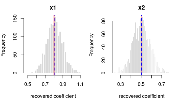
Each panel: the spread of one recovered coefficient across 1600 generated datasets. Red line = the true value, blue dashed = the average estimate. File reproduces from seed: yes.
log-odds(y = 1) = logit(0.30) + 0.5·x1 + 0.4·g[2] + 0.8·g[3]
R formula y ~ x1 + g · logistic regression (R’s glm) · n = 1000 ·
saved as data/glm_factor_a.rds
How it’s built: one continuous predictor (x1) drawn from a
standard normal (mean 0, sd 1); a 3-level factor g at proportions
50%/30%/20%. The outcome is 1 or 0, drawn at the logistic probability of
the formula above (baseline rate 30%). Sample size 1000, random seed
2137.
Data checks — statistics of the generated data, averaged over all draws, vs. what was requested:
| What we check | Requested | Average over draws | Allowed difference | Result |
|---|---|---|---|---|
| average of x1 | 0.0 | 0.0014 | within 0.01 | OK |
| std. deviation of x1 | 1.0 | 0.9996 | within 0.01 | OK |
| proportion in level 0 | 0.5 | 0.5000 | within 0.01 | OK |
| proportion in level 1 | 0.3 | 0.3000 | within 0.01 | OK |
| proportion in level 2 | 0.2 | 0.2000 | within 0.01 | OK |
Coefficient recovery — an independent R model fitted to each generated dataset; the average estimate should land on the true value:
| Term | True value | Recovered (average) | Spread across draws | Std. errors from true | Result |
|---|---|---|---|---|---|
| intercept | -0.8473 | -0.8505 | 0.1012 | -1.2502 | OK |
| x1 | 0.5000 | 0.5045 | 0.0715 | 2.4953 | OK |
| g[2] | 0.4000 | 0.3937 | 0.1585 | -1.5868 | OK |
| g[3] | 0.8000 | 0.8032 | 0.1816 | 0.6986 | OK |
Every coefficient is centred on its true value — the formula holds in the generated data.
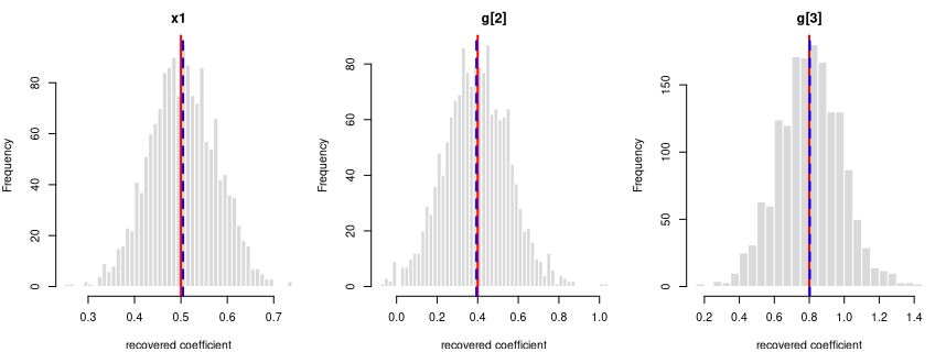
Each panel: the spread of one recovered coefficient across 1600 generated datasets. Red line = the true value, blue dashed = the average estimate. File reproduces from seed: yes.
log-odds(y = 1) = logit(0.50) + 0.8·x1 + 0.5·g[2] + 0.8·g[3]
R formula y ~ x1 + g · logistic regression (R’s glm) · n = 1000 ·
saved as data/glm_factor_b.rds
How it’s built: one continuous predictor (x1) drawn from a
standard normal (mean 0, sd 1); a 3-level factor g at proportions
40%/35%/25%. The outcome is 1 or 0, drawn at the logistic probability of
the formula above (baseline rate 50%). Sample size 1000, random seed
2138.
Data checks — statistics of the generated data, averaged over all draws, vs. what was requested:
| What we check | Requested | Average over draws | Allowed difference | Result |
|---|---|---|---|---|
| average of x1 | 0.00 | 0.0015 | within 0.01 | OK |
| std. deviation of x1 | 1.00 | 0.9996 | within 0.01 | OK |
| proportion in level 0 | 0.40 | 0.4000 | within 0.01 | OK |
| proportion in level 1 | 0.35 | 0.3500 | within 0.01 | OK |
| proportion in level 2 | 0.25 | 0.2500 | within 0.01 | OK |
Coefficient recovery — an independent R model fitted to each generated dataset; the average estimate should land on the true value:
| Term | True value | Recovered (average) | Spread across draws | Std. errors from true | Result |
|---|---|---|---|---|---|
| intercept | 0.0 | -0.0014 | 0.1077 | -0.5165 | OK |
| x1 | 0.8 | 0.8075 | 0.0792 | 3.7777 | OK |
| g[2] | 0.5 | 0.4983 | 0.1626 | -0.4064 | OK |
| g[3] | 0.8 | 0.8052 | 0.1771 | 1.1727 | OK |
Every coefficient is centred on its true value — the formula holds in the generated data.
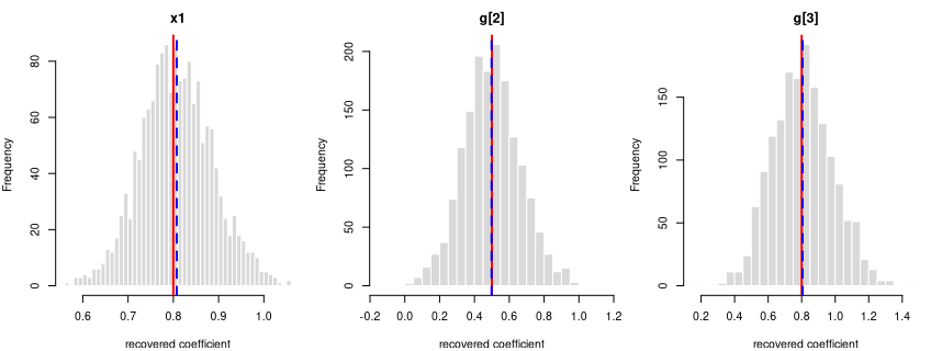
Each panel: the spread of one recovered coefficient across 1600 generated datasets. Red line = the true value, blue dashed = the average estimate. File reproduces from seed: yes.
log-odds(y = 1) = logit(0.30) + 0.5·x1 + 0.3·x2 + 0.3·x1:x2
R formula y ~ x1*x2 · logistic regression (R’s glm) · n = 1000 ·
saved as data/glm_interaction_a.rds
How it’s built: 2 continuous predictors (x1, x2) drawn from a
standard normal (mean 0, sd 1). The outcome is 1 or 0, drawn at the
logistic probability of the formula above (baseline rate 30%). Sample
size 1000, random seed 2137.
Data checks — statistics of the generated data, averaged over all draws, vs. what was requested:
| What we check | Requested | Average over draws | Allowed difference | Result |
|---|---|---|---|---|
| average of x1 | 0 | 0.0014 | within 0.01 | OK |
| std. deviation of x1 | 1 | 0.9996 | within 0.01 | OK |
| average of x2 | 0 | 0.0007 | within 0.01 | OK |
| std. deviation of x2 | 1 | 0.9993 | within 0.01 | OK |
Coefficient recovery — an independent R model fitted to each generated dataset; the average estimate should land on the true value:
| Term | True value | Recovered (average) | Spread across draws | Std. errors from true | Result |
|---|---|---|---|---|---|
| intercept | -0.8473 | -0.8532 | 0.0719 | -3.3004 | OK |
| x1 | 0.5000 | 0.5054 | 0.0767 | 2.8177 | OK |
| x2 | 0.3000 | 0.3033 | 0.0735 | 1.7887 | OK |
| x1:x2 | 0.3000 | 0.3008 | 0.0808 | 0.3714 | OK |
Every coefficient is centred on its true value — the formula holds in the generated data.
Each panel: the spread of one recovered coefficient across 1600 generated datasets. Red line = the true value, blue dashed = the average estimate. File reproduces from seed: yes.
log-odds(y = 1) = logit(0.50) + 0.8·x1 + 0.5·x2 + 0.4·x1:x2
R formula y ~ x1*x2 · logistic regression (R’s glm) · n = 1000 ·
saved as data/glm_interaction_b.rds
How it’s built: 2 continuous predictors (x1, x2) drawn from a
standard normal (mean 0, sd 1). The outcome is 1 or 0, drawn at the
logistic probability of the formula above (baseline rate 50%). Sample
size 1000, random seed 2138.
Data checks — statistics of the generated data, averaged over all draws, vs. what was requested:
| What we check | Requested | Average over draws | Allowed difference | Result |
|---|---|---|---|---|
| average of x1 | 0 | 0.0015 | within 0.01 | OK |
| std. deviation of x1 | 1 | 0.9996 | within 0.01 | OK |
| average of x2 | 0 | 0.0007 | within 0.01 | OK |
| std. deviation of x2 | 1 | 0.9993 | within 0.01 | OK |
Coefficient recovery — an independent R model fitted to each generated dataset; the average estimate should land on the true value:
| Term | True value | Recovered (average) | Spread across draws | Std. errors from true | Result |
|---|---|---|---|---|---|
| intercept | 0.0 | -0.0028 | 0.0702 | -1.6099 | OK |
| x1 | 0.8 | 0.8085 | 0.0819 | 4.1426 | OK |
| x2 | 0.5 | 0.5070 | 0.0761 | 3.6710 | OK |
| x1:x2 | 0.4 | 0.4021 | 0.0864 | 0.9811 | OK |
Every coefficient is centred on its true value — the formula holds in the generated data.
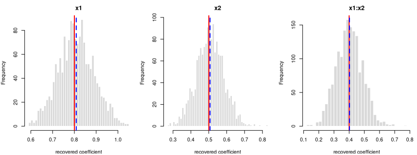
Each panel: the spread of one recovered coefficient across 1600 generated datasets. Red line = the true value, blue dashed = the average estimate. File reproduces from seed: yes.
y = 0.5·x1 + per-grp random intercept (ICC 0.20) + noise
R formula y ~ x1 + (1|grp) · linear mixed model (lme4::lmer) · n =
600 · saved as data/lme_simple_a.rds
How it’s built: one continuous predictor (x1) drawn from a
standard normal (mean 0, sd 1). The outcome is the formula above, plus a
shared offset for each of the 20 clusters (30 observations each, sized
to an intra-cluster correlation of 0.20), plus standard-normal noise.
Sample size 600, random seed 2137.
Data checks — statistics of the generated data, averaged over all draws, vs. what was requested:
| What we check | Requested | Average over draws | Allowed difference | Result |
|---|---|---|---|---|
| average of x1 | 0.0000 | 0.0007 | within 0.01 | OK |
| std. deviation of x1 | 1.0000 | 0.9993 | within 0.01 | OK |
| within-cluster variance | 1.0000 | 0.9990 | within 1% | OK |
| intra-cluster correlation (ICC) | 0.2000 | 0.1978 | within 0.01 | OK |
| observed (marginal) ICC vs predicted | 0.1659 | 0.1657 | within 0.01 | OK |
Coefficient recovery — an independent R model fitted to each generated dataset; the average estimate should land on the true value:
| Term | True value | Recovered (average) | Spread across draws | Std. errors from true | Result |
|---|---|---|---|---|---|
| intercept | 0.0 | 0.0085 | 0.1168 | 2.0682 | OK |
| x1 | 0.5 | 0.4992 | 0.0420 | -0.5401 | OK |
Every coefficient is centred on its true value — the formula holds in the generated data.
The intra-cluster correlation you set is the conditional ICC — the correlation between two observations in the same cluster after accounting for the predictors — and the generator recovers it (the “intra-cluster correlation (ICC)” row above). The observed (marginal) ICC of the raw outcome is lower, because the predictors explain part of the total variance; the stronger the fixed effects, the larger the gap. This is the standard conditional-vs-marginal distinction — expected and correct, not a generation fault — and the “observed (marginal) ICC vs predicted” row confirms the observed value lands on what that distinction predicts.
Each panel: the spread of one recovered coefficient across 800 generated datasets. Red line = the true value, blue dashed = the average estimate. File reproduces from seed: yes.
y = 0.3·x1 + per-grp random intercept (ICC 0.30) + noise
R formula y ~ x1 + (1|grp) · linear mixed model (lme4::lmer) · n =
600 · saved as data/lme_simple_b.rds
How it’s built: one continuous predictor (x1) drawn from a
standard normal (mean 0, sd 1). The outcome is the formula above, plus a
shared offset for each of the 20 clusters (30 observations each, sized
to an intra-cluster correlation of 0.30), plus standard-normal noise.
Sample size 600, random seed 2138.
Data checks — statistics of the generated data, averaged over all draws, vs. what was requested:
| What we check | Requested | Average over draws | Allowed difference | Result |
|---|---|---|---|---|
| average of x1 | 0.0000 | 0.0008 | within 0.01 | OK |
| std. deviation of x1 | 1.0000 | 0.9993 | within 0.01 | OK |
| within-cluster variance | 1.0000 | 0.9989 | within 1% | OK |
| intra-cluster correlation (ICC) | 0.3000 | 0.2948 | within 0.01 | OK |
| observed (marginal) ICC vs predicted | 0.2778 | 0.2779 | within 0.01 | OK |
Coefficient recovery — an independent R model fitted to each generated dataset; the average estimate should land on the true value:
| Term | True value | Recovered (average) | Spread across draws | Std. errors from true | Result |
|---|---|---|---|---|---|
| intercept | 0.0 | 0.0098 | 0.1491 | 1.8547 | OK |
| x1 | 0.3 | 0.2991 | 0.0421 | -0.5956 | OK |
Every coefficient is centred on its true value — the formula holds in the generated data.
The intra-cluster correlation you set is the conditional ICC — the correlation between two observations in the same cluster after accounting for the predictors — and the generator recovers it (the “intra-cluster correlation (ICC)” row above). The observed (marginal) ICC of the raw outcome is lower, because the predictors explain part of the total variance; the stronger the fixed effects, the larger the gap. This is the standard conditional-vs-marginal distinction — expected and correct, not a generation fault — and the “observed (marginal) ICC vs predicted” row confirms the observed value lands on what that distinction predicts.

Each panel: the spread of one recovered coefficient across 800 generated datasets. Red line = the true value, blue dashed = the average estimate. File reproduces from seed: yes.
y = 0.5·x1 + 0.3·x2 + per-grp random intercept (ICC 0.20) + noise
R formula y ~ x1 + x2 + (1|grp) · linear mixed model (lme4::lmer) ·
n = 750 · saved as data/lme_two_a.rds
How it’s built: 2 continuous predictors (x1, x2) drawn from a
standard normal (mean 0, sd 1). The outcome is the formula above, plus a
shared offset for each of the 25 clusters (30 observations each, sized
to an intra-cluster correlation of 0.20), plus standard-normal noise.
Sample size 750, random seed 2137.
Data checks — statistics of the generated data, averaged over all draws, vs. what was requested:
| What we check | Requested | Average over draws | Allowed difference | Result |
|---|---|---|---|---|
| average of x1 | 0.0000 | 0.0012 | within 0.01 | OK |
| std. deviation of x1 | 1.0000 | 0.9994 | within 0.01 | OK |
| average of x2 | 0.0000 | -0.0002 | within 0.01 | OK |
| std. deviation of x2 | 1.0000 | 0.9986 | within 0.01 | OK |
| within-cluster variance | 1.0000 | 0.9988 | within 1% | OK |
| intra-cluster correlation (ICC) | 0.2000 | 0.1978 | within 0.01 | OK |
| observed (marginal) ICC vs predicted | 0.1566 | 0.1549 | within 0.01 | OK |
Coefficient recovery — an independent R model fitted to each generated dataset; the average estimate should land on the true value:
| Term | True value | Recovered (average) | Spread across draws | Std. errors from true | Result |
|---|---|---|---|---|---|
| intercept | 0.0 | 0.0074 | 0.1073 | 1.9570 | OK |
| x1 | 0.5 | 0.4994 | 0.0380 | -0.4171 | OK |
| x2 | 0.3 | 0.3008 | 0.0372 | 0.6220 | OK |
Every coefficient is centred on its true value — the formula holds in the generated data.
The intra-cluster correlation you set is the conditional ICC — the correlation between two observations in the same cluster after accounting for the predictors — and the generator recovers it (the “intra-cluster correlation (ICC)” row above). The observed (marginal) ICC of the raw outcome is lower, because the predictors explain part of the total variance; the stronger the fixed effects, the larger the gap. This is the standard conditional-vs-marginal distinction — expected and correct, not a generation fault — and the “observed (marginal) ICC vs predicted” row confirms the observed value lands on what that distinction predicts.
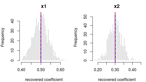
Each panel: the spread of one recovered coefficient across 800 generated datasets. Red line = the true value, blue dashed = the average estimate. File reproduces from seed: yes.
y = 0.3·x1 + 0.5·x2 + per-grp random intercept (ICC 0.30) + noise
R formula y ~ x1 + x2 + (1|grp) · linear mixed model (lme4::lmer) ·
n = 750 · saved as data/lme_two_b.rds
How it’s built: 2 continuous predictors (x1, x2) drawn from a
standard normal (mean 0, sd 1). The outcome is the formula above, plus a
shared offset for each of the 25 clusters (30 observations each, sized
to an intra-cluster correlation of 0.30), plus standard-normal noise.
Sample size 750, random seed 2138.
Data checks — statistics of the generated data, averaged over all draws, vs. what was requested:
| What we check | Requested | Average over draws | Allowed difference | Result |
|---|---|---|---|---|
| average of x1 | 0.0000 | 0.0012 | within 0.01 | OK |
| std. deviation of x1 | 1.0000 | 0.9994 | within 0.01 | OK |
| average of x2 | 0.0000 | -0.0001 | within 0.01 | OK |
| std. deviation of x2 | 1.0000 | 0.9986 | within 0.01 | OK |
| within-cluster variance | 1.0000 | 0.9988 | within 1% | OK |
| intra-cluster correlation (ICC) | 0.3000 | 0.2950 | within 0.01 | OK |
| observed (marginal) ICC vs predicted | 0.2395 | 0.2377 | within 0.01 | OK |
Coefficient recovery — an independent R model fitted to each generated dataset; the average estimate should land on the true value:
| Term | True value | Recovered (average) | Spread across draws | Std. errors from true | Result |
|---|---|---|---|---|---|
| intercept | 0.0 | 0.0088 | 0.1371 | 1.8113 | OK |
| x1 | 0.3 | 0.2994 | 0.0380 | -0.4832 | OK |
| x2 | 0.5 | 0.5009 | 0.0373 | 0.7116 | OK |
Every coefficient is centred on its true value — the formula holds in the generated data.
The intra-cluster correlation you set is the conditional ICC — the correlation between two observations in the same cluster after accounting for the predictors — and the generator recovers it (the “intra-cluster correlation (ICC)” row above). The observed (marginal) ICC of the raw outcome is lower, because the predictors explain part of the total variance; the stronger the fixed effects, the larger the gap. This is the standard conditional-vs-marginal distinction — expected and correct, not a generation fault — and the “observed (marginal) ICC vs predicted” row confirms the observed value lands on what that distinction predicts.
Each panel: the spread of one recovered coefficient across 800 generated datasets. Red line = the true value, blue dashed = the average estimate. File reproduces from seed: yes.
y = 0.5·x1 + 0.3·x2 + 0.3·x1:x2 + per-grp random intercept (ICC 0.20) + noise
R formula y ~ x1*x2 + (1|grp) · linear mixed model (lme4::lmer) · n
= 750 · saved as data/lme_interaction_a.rds
How it’s built: 2 continuous predictors (x1, x2) drawn from a
standard normal (mean 0, sd 1). The outcome is the formula above, plus a
shared offset for each of the 25 clusters (30 observations each, sized
to an intra-cluster correlation of 0.20), plus standard-normal noise.
Sample size 750, random seed 2137.
Data checks — statistics of the generated data, averaged over all draws, vs. what was requested:
| What we check | Requested | Average over draws | Allowed difference | Result |
|---|---|---|---|---|
| average of x1 | 0.0000 | 0.0012 | within 0.01 | OK |
| std. deviation of x1 | 1.0000 | 0.9994 | within 0.01 | OK |
| average of x2 | 0.0000 | -0.0002 | within 0.01 | OK |
| std. deviation of x2 | 1.0000 | 0.9986 | within 0.01 | OK |
| within-cluster variance | 1.0000 | 0.9988 | within 1% | OK |
| intra-cluster correlation (ICC) | 0.2000 | 0.1978 | within 0.01 | OK |
| observed (marginal) ICC vs predicted | 0.1485 | 0.1464 | within 0.01 | OK |
Coefficient recovery — an independent R model fitted to each generated dataset; the average estimate should land on the true value:
| Term | True value | Recovered (average) | Spread across draws | Std. errors from true | Result |
|---|---|---|---|---|---|
| intercept | 0.0 | 0.0075 | 0.1073 | 1.9725 | OK |
| x1 | 0.5 | 0.4994 | 0.0380 | -0.4690 | OK |
| x2 | 0.3 | 0.3008 | 0.0372 | 0.6211 | OK |
| x1:x2 | 0.3 | 0.3023 | 0.0363 | 1.8252 | OK |
Every coefficient is centred on its true value — the formula holds in the generated data.
The intra-cluster correlation you set is the conditional ICC — the correlation between two observations in the same cluster after accounting for the predictors — and the generator recovers it (the “intra-cluster correlation (ICC)” row above). The observed (marginal) ICC of the raw outcome is lower, because the predictors explain part of the total variance; the stronger the fixed effects, the larger the gap. This is the standard conditional-vs-marginal distinction — expected and correct, not a generation fault — and the “observed (marginal) ICC vs predicted” row confirms the observed value lands on what that distinction predicts.
Each panel: the spread of one recovered coefficient across 800 generated datasets. Red line = the true value, blue dashed = the average estimate. File reproduces from seed: yes.
y = 0.4·x1 + 0.3·x2 + 0.2·x1:x2 + per-grp random intercept (ICC 0.30) + noise
R formula y ~ x1*x2 + (1|grp) · linear mixed model (lme4::lmer) · n
= 900 · saved as data/lme_interaction_b.rds
How it’s built: 2 continuous predictors (x1, x2) drawn from a
standard normal (mean 0, sd 1). The outcome is the formula above, plus a
shared offset for each of the 30 clusters (30 observations each, sized
to an intra-cluster correlation of 0.30), plus standard-normal noise.
Sample size 900, random seed 2138.
Data checks — statistics of the generated data, averaged over all draws, vs. what was requested:
| What we check | Requested | Average over draws | Allowed difference | Result |
|---|---|---|---|---|
| average of x1 | 0.0000 | 0.0017 | within 0.01 | OK |
| std. deviation of x1 | 1.0000 | 0.9995 | within 0.01 | OK |
| average of x2 | 0.0000 | 0.0002 | within 0.01 | OK |
| std. deviation of x2 | 1.0000 | 0.9989 | within 0.01 | OK |
| within-cluster variance | 1.0000 | 1.0000 | within 1% | OK |
| intra-cluster correlation (ICC) | 0.3000 | 0.2958 | within 0.01 | OK |
| observed (marginal) ICC vs predicted | 0.2469 | 0.2462 | within 0.01 | OK |
Coefficient recovery — an independent R model fitted to each generated dataset; the average estimate should land on the true value:
| Term | True value | Recovered (average) | Spread across draws | Std. errors from true | Result |
|---|---|---|---|---|---|
| intercept | 0.0 | 0.0066 | 0.1240 | 1.4946 | OK |
| x1 | 0.4 | 0.3997 | 0.0345 | -0.2222 | OK |
| x2 | 0.3 | 0.3004 | 0.0344 | 0.3046 | OK |
| x1:x2 | 0.2 | 0.2025 | 0.0328 | 2.1481 | OK |
Every coefficient is centred on its true value — the formula holds in the generated data.
The intra-cluster correlation you set is the conditional ICC — the correlation between two observations in the same cluster after accounting for the predictors — and the generator recovers it (the “intra-cluster correlation (ICC)” row above). The observed (marginal) ICC of the raw outcome is lower, because the predictors explain part of the total variance; the stronger the fixed effects, the larger the gap. This is the standard conditional-vs-marginal distinction — expected and correct, not a generation fault — and the “observed (marginal) ICC vs predicted” row confirms the observed value lands on what that distinction predicts.
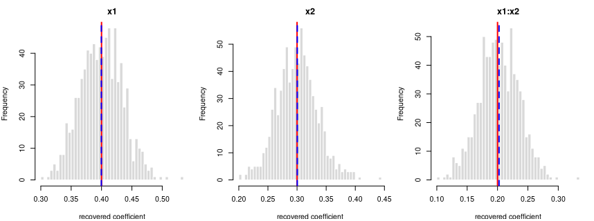
Each panel: the spread of one recovered coefficient across 800 generated datasets. Red line = the true value, blue dashed = the average estimate. File reproduces from seed: yes.
y = 0.3·x1 + 0.3·g[2] + per-grp random intercept (ICC 0.20) + noise
R formula y ~ x1 + g + (1|grp) · linear mixed model (lme4::lmer) · n
= 750 · saved as data/lme_factor_a.rds
How it’s built: one continuous predictor (x1) drawn from a
standard normal (mean 0, sd 1); a 2-level factor g at proportions
50%/50%. The outcome is the formula above, plus a shared offset for each
of the 25 clusters (30 observations each, sized to an intra-cluster
correlation of 0.20), plus standard-normal noise. Sample size 750,
random seed 2137.
Data checks — statistics of the generated data, averaged over all draws, vs. what was requested:
| What we check | Requested | Average over draws | Allowed difference | Result |
|---|---|---|---|---|
| average of x1 | 0.0000 | 0.0012 | within 0.01 | OK |
| std. deviation of x1 | 1.0000 | 0.9994 | within 0.01 | OK |
| proportion in level 0 | 0.5000 | 0.5000 | within 0.01 | OK |
| proportion in level 1 | 0.5000 | 0.5000 | within 0.01 | OK |
| within-cluster variance | 1.0000 | 0.9988 | within 1% | OK |
| intra-cluster correlation (ICC) | 0.2000 | 0.1978 | within 0.01 | OK |
| observed (marginal) ICC vs predicted | 0.1815 | 0.1806 | within 0.01 | OK |
Coefficient recovery — an independent R model fitted to each generated dataset; the average estimate should land on the true value:
| Term | True value | Recovered (average) | Spread across draws | Std. errors from true | Result |
|---|---|---|---|---|---|
| intercept | 0.0 | 0.0058 | 0.1142 | 1.4317 | OK |
| x1 | 0.3 | 0.2994 | 0.0380 | -0.4305 | OK |
| g[2] | 0.3 | 0.3033 | 0.0732 | 1.2911 | OK |
Every coefficient is centred on its true value — the formula holds in the generated data.
The intra-cluster correlation you set is the conditional ICC — the correlation between two observations in the same cluster after accounting for the predictors — and the generator recovers it (the “intra-cluster correlation (ICC)” row above). The observed (marginal) ICC of the raw outcome is lower, because the predictors explain part of the total variance; the stronger the fixed effects, the larger the gap. This is the standard conditional-vs-marginal distinction — expected and correct, not a generation fault — and the “observed (marginal) ICC vs predicted” row confirms the observed value lands on what that distinction predicts.
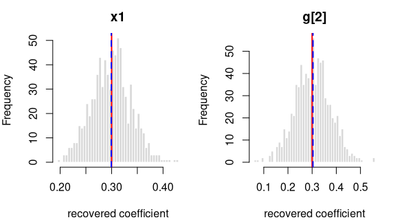
Each panel: the spread of one recovered coefficient across 800 generated datasets. Red line = the true value, blue dashed = the average estimate. File reproduces from seed: yes.
y = 0.4·x1 + 0.5·g[2] + 0.8·g[3] + per-grp random intercept (ICC 0.30) + noise
R formula y ~ x1 + g + (1|grp) · linear mixed model (lme4::lmer) · n
= 900 · saved as data/lme_factor_b.rds
How it’s built: one continuous predictor (x1) drawn from a
standard normal (mean 0, sd 1); a 3-level factor g at proportions
50%/30%/20%. The outcome is the formula above, plus a shared offset for
each of the 30 clusters (30 observations each, sized to an intra-cluster
correlation of 0.30), plus standard-normal noise. Sample size 900,
random seed 2138.
Data checks — statistics of the generated data, averaged over all draws, vs. what was requested:
| What we check | Requested | Average over draws | Allowed difference | Result |
|---|---|---|---|---|
| average of x1 | 0.0000 | 0.0017 | within 0.01 | OK |
| std. deviation of x1 | 1.0000 | 0.9995 | within 0.01 | OK |
| proportion in level 0 | 0.5000 | 0.5000 | within 0.01 | OK |
| proportion in level 1 | 0.3000 | 0.3000 | within 0.01 | OK |
| proportion in level 2 | 0.2000 | 0.2000 | within 0.01 | OK |
| within-cluster variance | 1.0000 | 1.0000 | within 1% | OK |
| intra-cluster correlation (ICC) | 0.3000 | 0.2958 | within 0.01 | OK |
| observed (marginal) ICC vs predicted | 0.3145 | 0.3136 | within 0.01 | OK |
Coefficient recovery — an independent R model fitted to each generated dataset; the average estimate should land on the true value:
| Term | True value | Recovered (average) | Spread across draws | Std. errors from true | Result |
|---|---|---|---|---|---|
| intercept | 0.0 | 0.0063 | 0.1779 | 1.0072 | OK |
| x1 | 0.4 | 0.3998 | 0.0345 | -0.1763 | OK |
| g[2] | 0.5 | 0.4928 | 0.2888 | -0.7017 | OK |
| g[3] | 0.8 | 0.8117 | 0.3162 | 1.0496 | OK |
Every coefficient is centred on its true value — the formula holds in the generated data.
The intra-cluster correlation you set is the conditional ICC — the correlation between two observations in the same cluster after accounting for the predictors — and the generator recovers it (the “intra-cluster correlation (ICC)” row above). The observed (marginal) ICC of the raw outcome is lower, because the predictors explain part of the total variance; the stronger the fixed effects, the larger the gap. This is the standard conditional-vs-marginal distinction — expected and correct, not a generation fault — and the “observed (marginal) ICC vs predicted” row confirms the observed value lands on what that distinction predicts.
Each panel: the spread of one recovered coefficient across 800 generated datasets. Red line = the true value, blue dashed = the average estimate. File reproduces from seed: yes.
How this was produced
| item | value |
|---|---|
| Report generated | 21 June 2026 |
| R version | R version 4.5.3 (2026-03-11) |
| mcpower | 1.0.0 |
| lme4 | 1.1.38 |
| Draws per formula (ordinary / logistic) | 1,600 |
| Draws per formula (mixed) | 800 |
| Recovery threshold | OLS/LME: pooled BH-FDR ≤ 0.001 (Benjamini-Hochberg); logit: |mean−true| ≤ 0.02 (absolute) |
| Formulas validated | 31 |
The datasets are generated by mcpower/validation/data_generation.r
from the formula catalogue in mcpower/validation/formulas.R; this
report regenerates them many times over and runs the checks above. To
reproduce it, from the repository root:
rmarkdown::render("mcpower/validation/validation_data_generation.rmd",
                  output_dir = "mcpower/web/documentation/validation")